A logic analyzer can show plausible protocol bytes and still miss the event that caused a failure. The usual reason is not the decoder; it is that the analyzer did not take enough samples across the shortest pulse. Sample rate must be chosen from the event width and signal bandwidth, not only from the advertised bus speed.
Digital logic analyzers commonly sample asynchronously: their sampling clock is independent of the target signal. If an input changes and changes back between two sample instants, the recorded trace may never show it. That is why a narrow chip-select glitch, interrupt pulse or enable strobe can disappear even when slower traffic looks correct.
Convert sample rate into time first
The sample interval is Ts = 1 ÷ Fs. At 1 MS/s, Ts is 1 µs. At 10 MS/s it is 100 ns, and at 100 MS/s it is 10 ns. Those intervals are easier to compare with a data-sheet pulse width than a large samples-per-second number.
Consider a 500 ns pulse captured at 1 MS/s. The analyzer checks the input once every 1 µs, so the entire pulse can fit between adjacent samples and remain invisible. Raising the rate to 10 MS/s places sample instants 100 ns apart, giving approximately five opportunities to record the pulse. The exact edge position still carries asynchronous timing uncertainty, but the event is no longer represented by zero or one ambiguous sample.
Use both bandwidth and minimum pulse width
Saleae recommends choosing a digital sample rate at least four times the signal bandwidth. A 10 MHz digital signal therefore calls for at least 40 MS/s under that rule. For analog channels, the company recommends at least ten times the recorded analog bandwidth.
The bandwidth rule is a starting point, not a guarantee for every waveform. A 1 MHz clock with a 50% duty cycle has 500 ns high and low intervals. A 1 MHz signal containing a 50 ns strobe has a much shorter event even though its repetition rate is low. The capture plan must satisfy whichever requirement is stricter: the signal-bandwidth multiple or enough samples across the minimum pulse width.
For a 100 kHz square wave at 1 MS/s, the analyzer records about ten samples per 10 µs cycle and roughly five per half-cycle. That may be adequate for protocol state, but it does not provide precise edge timing. Increasing the rate narrows the quantization interval: two edges each located only to the nearest 1 µs sample can make a short pulse-width measurement uncertain by roughly a sample interval at each boundary.
Channel count can change the available rate
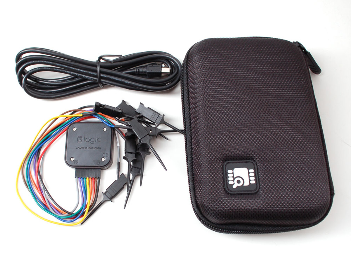
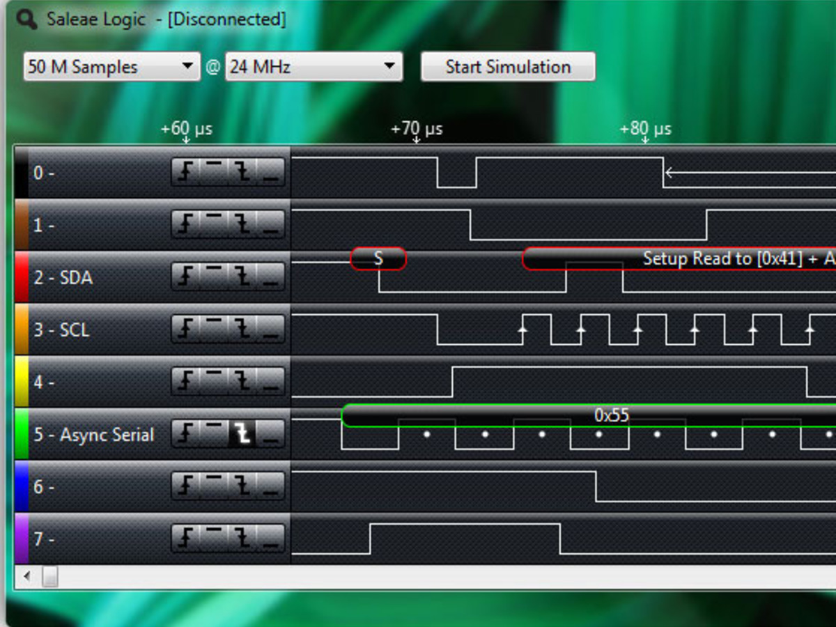
Do not assume the rate shown for one channel remains available after enabling every line. Saleae documents that Logic 8 supports 100 MS/s with up to three digital channels, 50 MS/s with up to six, and 40 MS/s with up to seven. Enabling analog channels changes the available combinations again.
This matters during escalation. A capture may begin with clock, data and chip select at 100 MS/s. Adding reset, interrupt, power-good and enable signals can push the device to a lower maximum. If the shortest event required the original rate, the expanded trace can become less trustworthy precisely when more context was added.
Plan the capture around the fault
Write down the fastest clock, the narrowest documented or suspected pulse, and the channels needed to explain the fault. Convert each candidate rate to its sample interval. Then check the actual software configuration after every channel change rather than relying on the device’s headline maximum.
Long captures create another tradeoff: rate multiplied by time and active channels determines data volume. Triggering on an error condition, recording fewer channels, or capturing a shorter window can preserve the required timing resolution without producing an unmanageable file.
If a decoder fails while edges look clean, compare its mode and threshold settings with the bus specification; SPI polarity and phase errors can produce wrong bytes without a sampling shortage. If a one-off pulse is absent, however, start with Ts. A trace cannot decode an event it never sampled.